
Office work with Excel will sooner or later have you staring at a column of mixed-case text wondering how to fix it without going cell by cell. Changing lowercase to uppercase manually is fine for five rows, but when you have hundreds or thousands of entries, you need a better way. In this article I will show you all the methods I know, from a custom shortcut key all the way to Power Query, so you can pick whichever fits your situation best.
Use the change lowercase to uppercase shortcut in Excel
Add the shortcut to Excel
First, download the PERSONAL.XLSB file from Lucid Gen. This file uses VBA to add a keyboard shortcut for changing letter case directly in Excel. I already did all the VBA work so you just need to drop the file in the right folder.
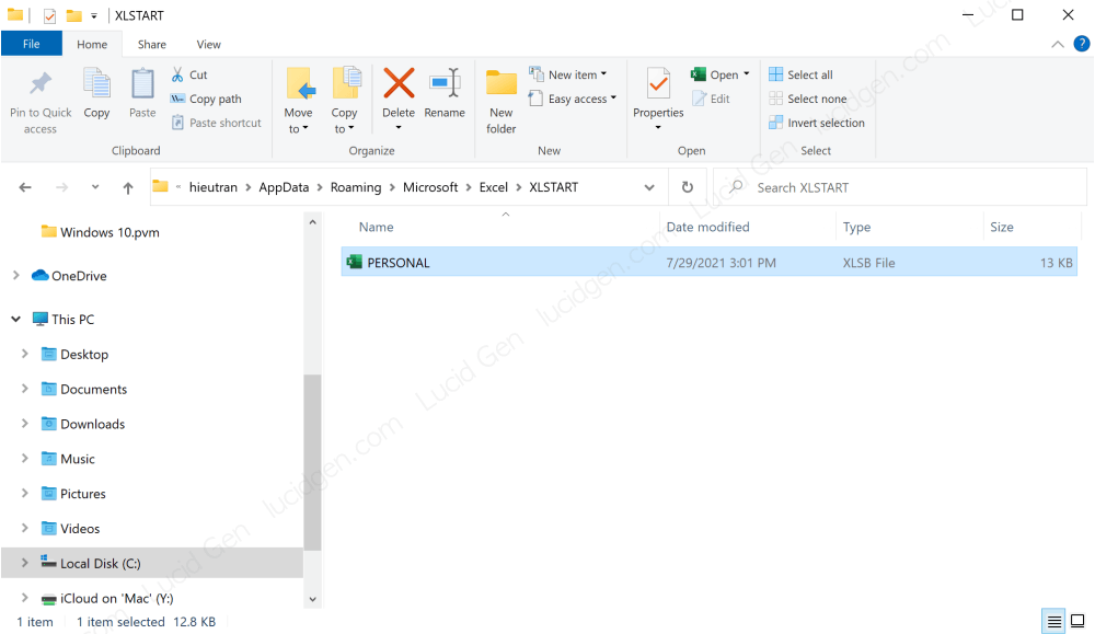
After downloading, place the PERSONAL.XLSB file into the XLSTART folder at this path:
C:Users/user-name/AppData/Roaming/Microsoft/Excel/XLSTARTIf you cannot find the AppData folder, it is hidden by default. To show it, open File Explorer, click VIEW > Options > View > enable “Show hidden files, folders, and drives” > Apply and OK.

Place the PERSONAL.XLSB file into the XLSTART folder like this.
Use the shortcut keys
Open a new Excel file and select the cells you want to convert. Then use these shortcuts:
- Ctrl J: convert to ALL CAPS (LUCID GEN)
- Ctrl M: capitalize the first letter of each word (Lucid Gen)
- Ctrl Q: convert to lowercase (lucid gen)

This works reliably on new Excel files. For older files that already have VBA in them, it may occasionally not work, but for everyday data sheets it is perfectly fine.
How to change lowercase to uppercase in Excel with formulas
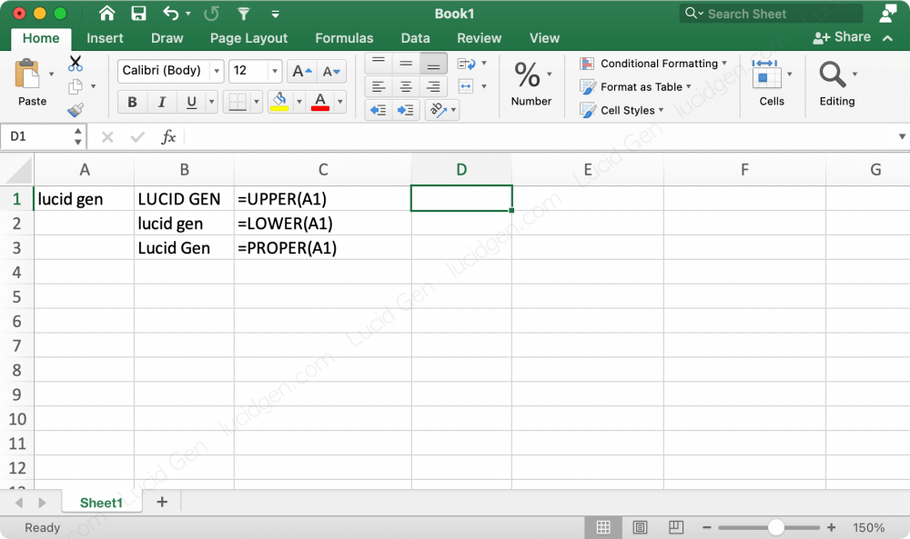
If you prefer not to install any file, Excel has three built-in functions for changing text case. For example, if cell A1 contains “lucid gen”, here is what each formula does:
| A | Formula | Result | |
| 1 | lucid gen | =UPPER(A1) | LUCID GEN |
| 2 | =LOWER(A1) | lucid gen | |
| 3 | =PROPER(A1) | Lucid Gen |
One thing to keep in mind with the formula method: the result is a formula, not plain text. If you want to replace the original column with converted text, copy the formula results, then use Paste Special > Values Only to paste them back. This removes the formula and keeps just the text, so you can safely delete the helper column.
Also note that PROPER() has a known quirk: it capitalizes the first letter after every space and every apostrophe. This can produce odd results with names like “McDonald” (it becomes “Mcdonald”) or abbreviations. For those cases, you may need to fix a few cells manually after running PROPER().
Use Flash Fill to change case (Excel 2013 and later)
Flash Fill is one of Excel’s most underrated features and it works great for case conversion too, especially if you just need a quick one-time fix without writing any formula.
Here is how it works. Say column A has your original lowercase text. In column B, type the uppercase version of the first cell manually. Then in the second row of column B, start typing. Excel will detect the pattern and suggest the rest of the column in grey. Press Enter to accept the suggestion and Flash Fill fills everything in one shot.
You can also trigger Flash Fill manually by pressing Ctrl + E, or going to Data > Flash Fill in the ribbon.
Flash Fill works best for clean, consistent data. If your source column has a lot of variation in format, the formula method or Power Query will give more reliable results.
Use Power Query for large data sets (Excel 2016 and later)
If you are working with large amounts of data or need to clean up case as part of a repeatable import process, Power Query is the most powerful option.
To use Power Query, select your data range, then go to Data > From Table/Range. In the Power Query editor, select the column you want to convert. Go to Transform > Format and choose UPPERCASE, lowercase, or Capitalize Each Word depending on what you need. Then click Close and Load to send the cleaned data back to your sheet.
The real advantage of Power Query is that the steps are saved. Next time you get a new batch of data, you just refresh the query and all the transformations run automatically. For recurring reports or regular data imports, this saves a lot of repetitive work.
Which method should you use?
Here is a quick summary to help you pick the right approach for your situation.
Use the shortcut key (PERSONAL.XLSB) if you convert case frequently throughout your workday and want the fastest possible workflow. One keystroke and done, no helper column needed.
Use UPPER / LOWER / PROPER formulas if you need a no-setup solution or are on a shared computer where you cannot install files. It is the most universally available method.
Use Flash Fill if you have a one-time task and want something quick without any formulas. Great for small to medium sized data.
Use Power Query if you have large data sets or need to repeat the same cleaning steps regularly. The best option for systematic data processing workflows.
A note for Excel on Mac
The PERSONAL.XLSB shortcut method described in this article is designed for Excel on Windows. If you are using Excel on Mac, the XLSTART folder path is different and the keyboard shortcuts may conflict with macOS system shortcuts.
On Mac, the XLSTART folder is located at: Users/your-username/Library/Group Containers/UBF8T346G9.Office/User Content/Excel/XLSTART. You can place the PERSONAL.XLSB file there, but you may need to reassign the shortcut keys if Ctrl+J, Ctrl+M, or Ctrl+Q are already in use by macOS.
The formula method (UPPER, LOWER, PROPER) and Flash Fill work identically on both Windows and Mac, so those are the easiest cross-platform options.
Conclusion
Using the PERSONAL.XLSB shortcut has genuinely made my data entry work in Excel noticeably faster, no more formula columns and copy-paste-special routines just to fix some text case. Give it a try and let me know in the comments how it goes for you. And if you prefer staying formula-based, UPPER() and LOWER() are always there for you.


