

In recruitment and many other fields, we often use Google Forms to collect candidate or customer data. The responses are saved to Google Sheets, which works much like Excel, so duplicate data is almost impossible to avoid. So how do you find duplicates in Google Sheets? For Excel, you can easily find solutions online, but filtering works a bit differently in Google Sheets. In this post, I’ll share the methods I use.

The list above contains many duplicate names. You can find and filter duplicates in several ways, depending on what you need.
Highlight duplicates in Google Sheets
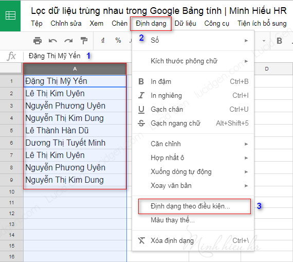
To find duplicate data in Google Sheets, select the column that contains your data. Click Format and select Conditional formatting.
In the Conditional format rules panel, enter the formula as shown below.
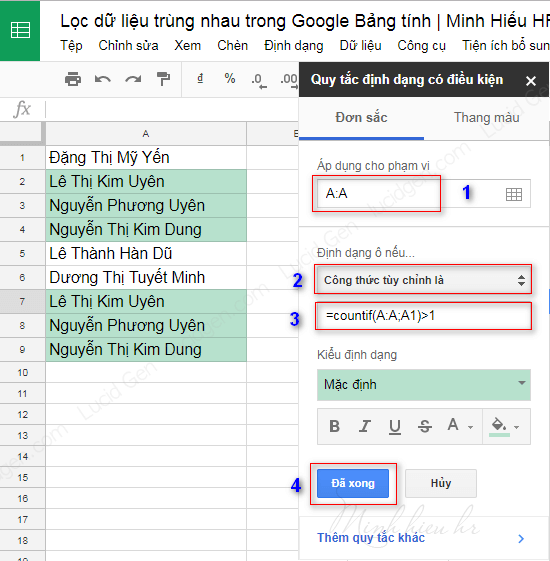
=Countif(A:A;A1)>1
Note: if the semicolon doesn’t work on your device, change it to a comma. Also replace the letter A with the letter of the column you’re formatting in your file.
Now you can easily spot the duplicate data, so the next step is to filter it. There are 2 ways to filter duplicates in Google Sheets.
Filter duplicate or unique values
I inserted a row at the top for the column headers. In the first cell next to your data, enter the formula shown below, then drag it down the entire column.

=countif(A:A;A2)=1
Now TRUE marks values that are not duplicated, and FALSE marks values that are. Click row number 1 to select the header row, click Data, and select Create a filter.
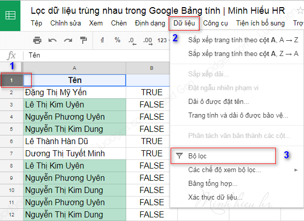
Next, click the filter button. If you want to see the unique values, keep TRUE. If you want to see the duplicates, keep FALSE.

Here’s the result when we keep TRUE, which means only the unique values.
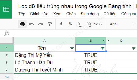
But this method isn’t ideal, because you can only see values that are duplicated or not. What we really want is the full list of data, with only the repeated occurrences (the second time onwards) filtered out.
Filter out values from their second occurrence
Select the first cell next to the data column. I chose column B, so the cell next to A2 is B2. In this cell, enter the formula shown below.
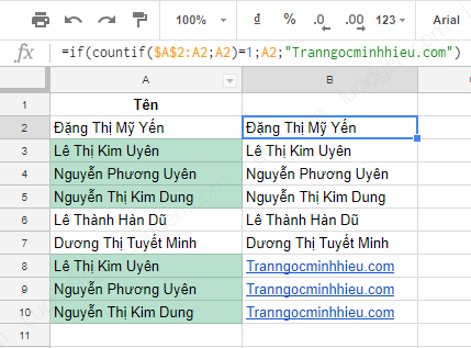
Now every cell that repeats for the second time or more will show Tranngocminhhieu.com.
=if(countif($A$2:A2;A2)=1;A2;”Tranngocminhhieu.com”)
Explanation:
$A$2: an absolute reference that stays fixed
A2: a relative reference that changes as you drag down
“Tranngocminhhieu.com”: you can write whatever you want here
To keep only the first occurrence of each value, click the filter button > uncheck Tranngocminhhieu.com > OK.

Pretty neat, right?

As a result, you have a complete list without losing any data and without any duplicates. You can also see which values were duplicated in the highlighted cells.
Remove duplicate data in Google Sheets
Google Sheets now has a built-in feature to remove duplicates. Just select the column you want to clean up > Data > Data cleanup > Remove duplicates.

Conclusion
The last filtering method is handy for many tasks, such as sending bulk emails or messages to a clean list. Here’s another related article you might find useful: merging multiple Excel and CSV files into 1 Sheet. What do you think about the methods above, and did you run into any difficulties? Let me know in the comments below.


